How the project evolved
This sequence is important to me because the final models make more sense when I remember why each step happened.
We quantified class imbalance, tiny defect areas, category variation and spatial structure, and documented that first investigation in the MVTec AD EDA Report. Those findings led us to question accuracy and pixel AUROC as primary metrics and shaped the modelling phase that followed.
An early simple baseline tested whether pretrained features could separate normality without training a task-specific network.
We learned reconstruction-based anomaly detection, experimented with bottlenecks, masked regions, reconstruction losses and image-level scoring.
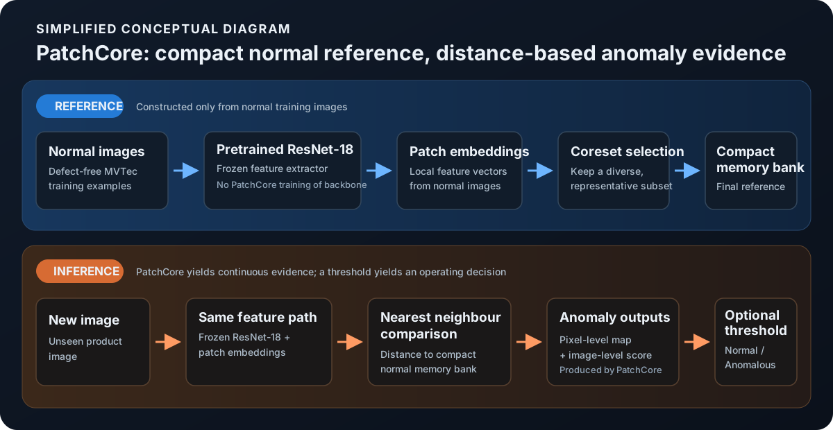
We moved from reconstructing pixels to matching local pretrained patch embeddings against a compact normal memory bank.
We discovered that historical PatchCore and CAE results had not followed identical fitting, calibration and pixel-metric paths, so the comparison needed correction.
fair-eval-v1.One deterministic split, validation-only thresholds, common ordered test sets, common pixel canonicalization, shared metric implementations and versioned artifacts.
Frozen self-supervised ViT patch tokens became a normal feature bank; nearest-neighbour patch distance produced image scores and dense anomaly maps.
I tested multiple layers, position-aware 5-NN, local-density normalization and PatchCore-style aggregation. Some pixel metrics improved, but the primary image decision became worse.
The same fair scorer was applied to a frozen DINOv3 encoder. It slightly weakened image decisions but produced the strongest mean AUPIMO in the repository comparison.
Model primers: what each approach is actually doing
Convolutional autoencoder: detect what cannot be reconstructed normally
A convolutional autoencoder compresses an image through an encoder and reconstructs it through a decoder. Trained only on good parts, the intuition is that normal structure should reconstruct well while unfamiliar defects leave larger reconstruction errors.
image → encoder → bottleneck → decoder → reconstruction → error mapOur experiments included masked reconstruction and alternative scoring strategies. The main practical difficulty was that reconstruction error is not defect-specific: complex textures, blur, small spatial shifts and decoder smoothing can produce high error on perfectly normal areas. That made reconstruction-based approaches much weaker than feature-matching methods in the final comparison.
PatchCore: remember normal local features instead of reconstructing pixels
PatchCore uses a frozen pretrained CNN to extract local patch embeddings from normal images. A coreset compresses those embeddings into a memory bank. During inference, each test patch is scored by its distance to the nearest normal reference patch.
DINOv2 / DINOv3: the same normal-memory idea with self-supervised ViT patch tokens
DINO models give a patch-level representation from a frozen Vision Transformer. Our simple baseline stores normal patch tokens and scores a query patch by 1-nearest-neighbour distance. The strength of the representation meant that a comparatively simple anomaly scorer could outperform the more complicated pipelines at image level.
image → frozen ViT → patch tokens → normal feature bank → 1-NN distances → anomaly map + image scoreFinal repository comparison
All values below are unweighted macro means across the 15 categories under fair-eval-v1. Image F1 was treated as the primary deployed image-decision metric; PR-AUC gives threshold-independent image-level context; AUPIMO measures low-false-positive localization.
| Model | Image F1 | Image PR-AUC | AUPIMO | Reading |
|---|---|---|---|---|
| DINOv2, single-layer 1-NN | 0.941 | 0.989 | 0.602 | Strongest image decision |
| DINOv3, single-layer 1-NN | 0.932 | 0.986 | 0.680 | Strongest low-FPR localization |
| PatchCore | 0.929 | 0.988 | 0.603 | Strong, mature feature-memory baseline |
| DINOv2, enhanced | 0.920 | 0.983 | 0.545 | More complex, worse primary decision |
| Keras CAE | 0.495 | 0.867 | 0.058 | Reconstruction approach lagged badly |
The enhanced DINOv2 experiment is a useful warning against assuming that “more sophisticated” means “better.” Multi-layer features, position-aware 5-NN, local-density normalization and PatchCore-style aggregation improved mean pixel F1 from 0.290 to 0.385 and pixel AUROC from 0.969 to 0.979, but mean image F1 fell from 0.941 to 0.920 and AUPIMO from 0.602 to 0.545.
DINOv3 also requires careful interpretation. It improved mean AUPIMO to 0.680, but its masking configuration was not identical: the DINOv2 masking rule could produce an empty DINOv3 memory bank, so DINOv3 was evaluated with masking disabled. The full AUPIMO gain therefore cannot be attributed to the encoder alone.
What failed, or nearly fooled us
When anomalous pixels are tiny, predicting almost everything as normal can look numerically excellent while detecting no useful defect geometry.
Autoencoders can produce high residuals on legitimate texture detail, blur or slight shifts, especially on stochastic surfaces.
The same ranking model can look precise or recall-heavy depending on the cutoff. Thresholding is an operating decision, not an afterthought.
Different train membership, calibration data or pixel metric implementations can change conclusions even when the model code itself is unchanged.
Rotation, greyscale presentation and small localized defects made screw a recurring failure case and motivated targeted exploration.
The enhanced DINOv2 maps improved on some pixel metrics while image F1 and AUPIMO worsened.
For more qualitative examples and category-level PatchCore behavior, see the dedicated evaluation page.